Let's learn, share & inspire each other. Sign up now 🤘🏼
Let's learn, share & inspire each other. Sign up now 🤘🏼
 ARTICLE
 52 min read
A Comprehensive Hands-on Guide to Transfer Learning with Real-World Applications in Deep Learning
Humans have an inherent ability to transfer knowledge across tasks. What we acquire as knowledge while learning about one task, we utilize in the same way to solve related tasks. The more related the tasks, the easier it is for us to transfer, or cross-utilize our knowledge. Some simple examples would be,
In each of the above scenarios, we don’t learn everything from scratch when we attempt to learn new aspects or topics. We transfer and leverage our knowledge from what we have learnt in the past!
Conventional machine learning and deep learning algorithms, so far, have been traditionally designed to work in isolation. These algorithms are trained to solve specific tasks. The models have to be rebuilt from scratch once the feature-space distribution changes. Transfer learning is the idea of overcoming the isolated learning paradigm and utilizing knowledge acquired for one task to solve related ones. In this article, we will do a comprehensive coverage of the concepts, scope and real-world applications of transfer learning and even showcase some hands-on examples. To be more specific, we will be covering the following.
We will look at transfer learning as a general high-level concept which started right from the days of machine learning and statistical modeling, however, we will be more focused around deep learning in this article.
This article aims to be an attempt to cover theoretical concepts as well as demonstrate practical hands-on examples of deep learning applications in one place, given the information overload which is out there on the web. All examples will be covered in Python using keras with a tensorflow backend, a perfect match for people who are veterans or just getting started with deep learning!
We have already briefly discussed that humans don’t learn everything from the ground up and leverage and transfer their knowledge from previously learnt domains to newer domains and tasks. Given the craze for True Artificial General Intelligence, transfer learning is something which data scientists and researchers believe can further our progress towards AGI. After supervised learning — Transfer Learning will be the next driver of ML commercial success
In fact, transfer learning is not a concept which just cropped up in the 2010s. The Neural Information Processing Systems (NIPS) 1995 workshop Learning to Learn: Knowledge Consolidation and Transfer in Inductive Systems is believed to have provided the initial motivation for research in this field. Since then, terms such as Learning to Learn, Knowledge Consolidation, and Inductive Transfer have been used interchangeably with transfer learning. Invariably, different researchers and academic texts provide definitions from different contexts. In their famous book, Deep Learning, Goodfellow et al refer to transfer learning in the context of generalization. Their definition is as follows:
Situation where what has been learned in one setting is exploited to improve generalization in another setting.
Thus, the key motivation, especially considering the context of deep learning is the fact that most models which solve complex problems need a whole lot of data, and getting vast amounts of labeled data for supervised models can be really difficult, considering the time and effort it takes to label data points. A simple example would be the ImageNet dataset, which has millions of images pertaining to different categories, thanks to years of hard work starting at Stanford!

The popular ImageNet Challenge based on the ImageNet Database
However, getting such a dataset for every domain is tough. Besides, most deep learning models are very specialized to a particular domain or even a specific task. While these might be state-of-the-art models, with really high accuracy and beating all benchmarks, it would be only on very specific datasets and end up suffering a significant loss in performance when used in a new task which might still be similar to the one it was trained on. This forms the motivation for transfer learning, which goes beyond specific tasks and domains, and tries to see how to leverage knowledge from pre-trained models and use it to solve new problems!
The first thing to remember here is that, transfer learning, is not a new concept which is very specific to deep learning. There is a stark difference between the traditional approach of building and training machine learning models, and using a methodology following transfer learning principles.

Traditional Learning vs Transfer Learning
Traditional learning is isolated and occurs purely based on specific tasks, datasets and training separate isolated models on them. No knowledge is retained which can be transferred from one model to another. In transfer learning, you can leverage knowledge (features, weights etc) from previously trained models for training newer models and even tackle problems like having less data for the newer task!
Let’s understand the preceding explanation with the help of an example. Let’s assume our task is to identify objects in images within a restricted domain of a restaurant. Let’s mark this task in its defined scope as T1. Given the dataset for this task, we train a model and tune it to perform well (generalize) on unseen data points from the same domain (restaurant). Traditional supervised ML algorithms break down when we do not have sufficient training examples for the required tasks in given domains. Suppose, we now must detect objects from images in a park or a café (say, task T2). Ideally, we should be able to apply the model trained for T1, but in reality, we face performance degradation and models that do not generalize well. This happens for a variety of reasons, which we can liberally and collectively term as the model’s bias towards training data and domain.
Transfer learning should enable us to utilize knowledge from previously learned tasks and apply them to newer, related ones. If we have significantly more data for task T1, we may utilize its learning, and generalize this knowledge (features, weights) for task T2 (which has significantly less data). In the case of problems in the computer vision domain, certain low-level features, such as edges, shapes, corners and intensity, can be shared across tasks, and thus enable knowledge transfer among tasks! Also, as we have depicted in the earlier figure, knowledge from an existing task acts as an additional input when learning a new target task.
Let’s now take a look at a formal definition for transfer learning and then utilize it to understand different strategies. In their paper, A Survey on Transfer Learning, Pan and Yang use domain, task, and marginal probabilities to present a framework for understanding transfer learning. The framework is defined as follows:
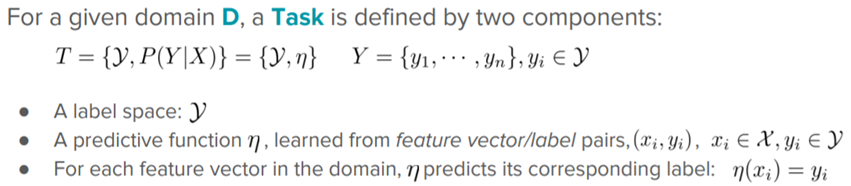
A domain, D, is defined as a two-element tuple consisting of feature space, ꭕ, and marginal probability, P(Χ), where Χ is a sample data point. Thus, we can represent the domain mathematically as D = {ꭕ, P(Χ)}

Here xᵢ represents a specific vector as represented in the above depiction. A task, T, on the other hand, can be defined as a two-element tuple of the label space, γ, and objective function, η. The objective function can also be denoted as P(γ| Χ) from a probabilistic view point.
Thus, armed with these definitions and representations, we can define transfer learning as follows:

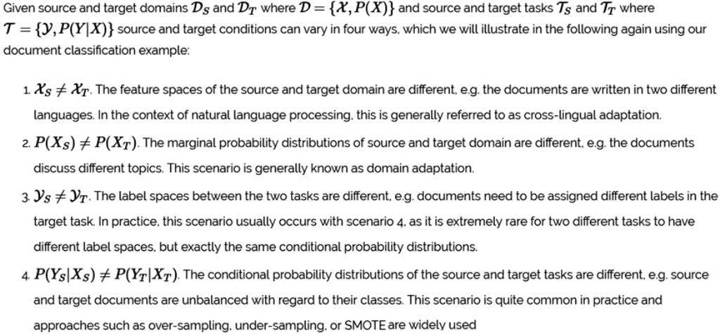
Let’s now take a look at the typical scenarios involving transfer learning based on our previous definition.
To give some more clarity on the difference between the terms domain and task, the following figure tries to explain them with some examples.

Transfer learning, as we have seen so far, is having the ability to utilize existing knowledge from the source learner in the target task. During the process of transfer learning, the following three important questions must be answered:
This should help us define the various scenarios where transfer learning can be applied and possible techniques, which we will discuss in the next section.
There are different transfer learning strategies and techniques, which can be applied based on the domain, task at hand, and the availability of data. I really like the following figure from the paper on transfer learning we mentioned earlier, A Survey on Transfer Learning.

Transfer Learning Strategies
Thus, based on the previous figure, transfer learning methods can be categorized based on the type of traditional ML algorithms involved, such as:
We can summarize the different settings and scenarios for each of the above techniques in the following table.
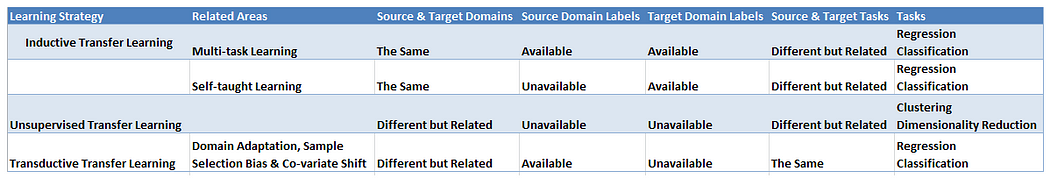
Types of Transfer Learning Strategies and their Settings
The three transfer categories discussed in the previous section outline different settings where transfer learning can be applied, and studied in detail. To answer the question of what to transfer across these categories, some of the following approaches can be applied:
The following table clearly summarizes the relationship between different transfer learning strategies and what to transfer.
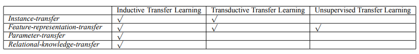
Transfer Learning Strategies and Types of Transferable Components
Let’s now utilize this understanding and learn how transfer learning is applied in the context of deep learning.
The strategies we discussed in the previous section are general approaches which can be applied towards machine learning techniques, which brings us to the question, can transfer learning really be applied in the context of deep learning?
Deep learning models are representative of what is also known as inductive learning. The objective for inductive-learning algorithms is to infer a mapping from a set of training examples. For instance, in cases of classification, the model learns mapping between input features and class labels. In order for such a learner to generalize well on unseen data, its algorithm works with a set of assumptions related to the distribution of the training data. These sets of assumptions are known as inductive bias. The inductive bias or assumptions can be characterized by multiple factors, such as the hypothesis space it restricts to and the search process through the hypothesis space. Thus, these biases impact how and what is learned by the model on the given task and domain.

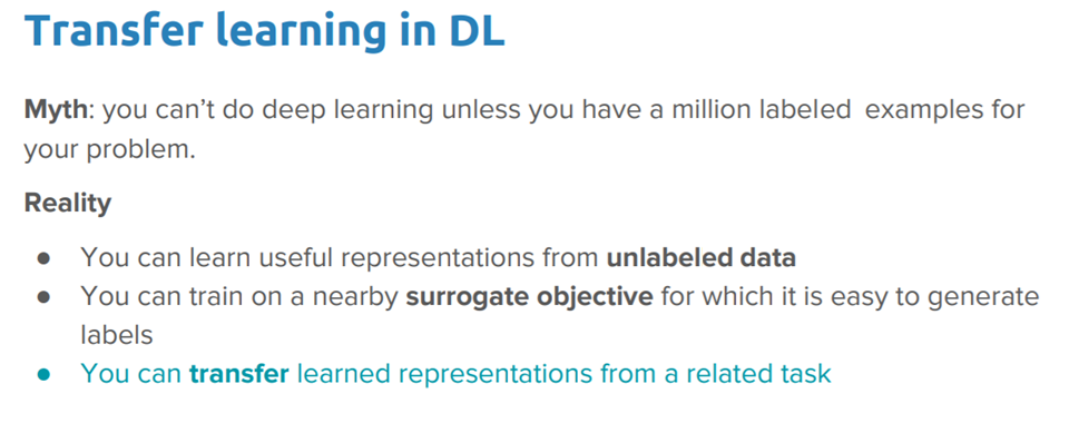
Ideas for deep transfer learning
Inductive transfer techniques utilize the inductive biases of the source task to assist the target task. This can be done in different ways, such as by adjusting the inductive bias of the target task by limiting the model space, narrowing down the hypothesis space, or making adjustments to the search process itself with the help of knowledge from the source task. This process is depicted visually in the following figure.
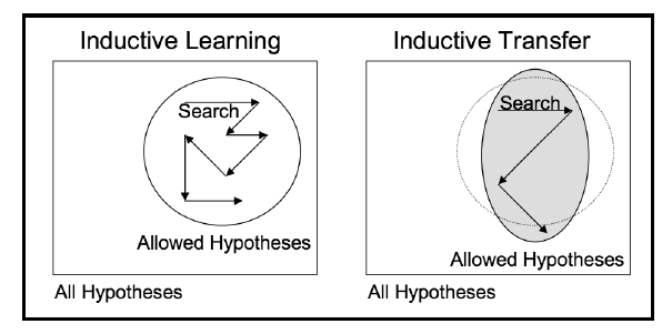
Inductive transfer (Source: Transfer learning, Lisa Torrey and Jude Shavlik)
Apart from inductive transfer, inductive-learning algorithms also utilize Bayesian and Hierarchical transfer techniques to assist with improvements in the learning and performance of the target task.
Deep learning has made considerable progress in recent years. This has enabled us to tackle complex problems and yield amazing results. However, the training time and the amount of data required for such deep learning systems are much more than that of traditional ML systems. There are various deep learning networks with state-of-the-art performance (sometimes as good or even better than human performance) that have been developed and tested across domains such as computer vision and natural language processing (NLP). In most cases, teams/people share the details of these networks for others to use. These pre-trained networks/models form the basis of transfer learning in the context of deep learning, or what I like to call ‘deep transfer learning’. Let’s look at the two most popular strategies for deep transfer learning.
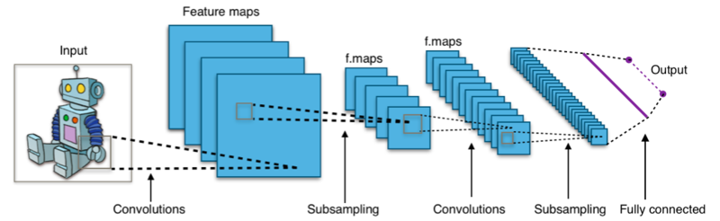
Deep learning systems and models are layered architectures that learn different features at different layers (hierarchical representations of layered features). These layers are then finally connected to a last layer (usually a fully connected layer, in the case of supervised learning) to get the final output. This layered architecture allows us to utilize a pre-trained network (such as Inception V3 or VGG) without its final layer as a fixed feature extractor for other tasks.
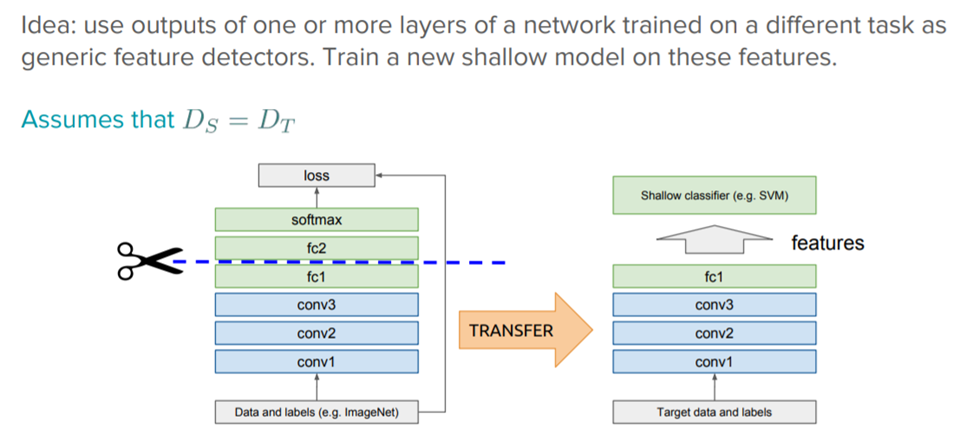
Transfer Learning with Pre-trained Deep Learning Models as Feature Extractors
The key idea here is to just leverage the pre-trained model’s weighted layers to extract features but not to update the weights of the model’s layers during training with new data for the new task.
For instance, if we utilize AlexNet without its final classification layer, it will help us transform images from a new domain task into a 4096-dimensional vector based on its hidden states, thus enabling us to extract features from a new domain task, utilizing the knowledge from a source-domain task. This is one of the most widely utilized methods of performing transfer learning using deep neural networks.
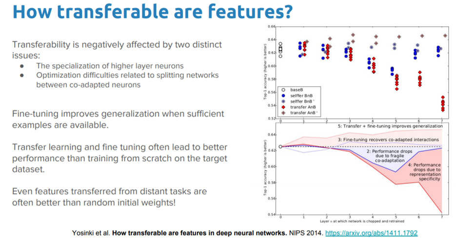
Now a question might arise, how well do these pre-trained off-the-shelf features really work in practice with different tasks?

It definitely seems to work really well in real-world tasks, and if the chart in the above table is not very clear, the following figure should make things more clear with regard to their performance in different computer vision based tasks!

Performance of off-the-shelf pre-trained models vs. specialized task-focused deep learning models
Based on the red and pink bars in the above figure, you can clearly see that the features from the pre-trained models consistently out-perform very specialized task-focused deep learning models.
This is a more involved technique, where we do not just replace the final layer (for classification/regression), but we also selectively retrain some of the previous layers. Deep neural networks are highly configurable architectures with various hyperparameters. As discussed earlier, the initial layers have been seen to capture generic features, while the later ones focus more on the specific task at hand. An example is depicted in the following figure on a face-recognition problem, where initial lower layers of the network learn very generic features and the higher layers learn very task-specific features.

Using this insight, we may freeze (fix weights) certain layers while retraining, or fine-tune the rest of them to suit our needs. In this case, we utilize the knowledge in terms of the overall architecture of the network and use its states as the starting point for our retraining step. This, in turn, helps us achieve better performance with less training time.

This brings us to the question, should we freeze layers in the network to use them as feature extractors or should we also fine-tune layers in the process?

This should give us a good perspective on what each of these strategies are and when should they be used!
One of the fundamental requirements for transfer learning is the presence of models that perform well on source tasks. Luckily, the deep learning world believes in sharing. Many of the state-of-the art deep learning architectures have been openly shared by their respective teams. These span across different domains, such as computer vision and NLP, the two most popular domains for deep learning applications. Pre-trained models are usually shared in the form of the millions of parameters/weights the model achieved while being trained to a stable state. Pre-trained models are available for everyone to use through different means. The famous deep learning Python library, keras, provides an interface to download some popular models. You can also access pre-trained models from the web since most of them have been open-sourced.
For computer vision, you can leverage some popular models including,
For natural language processing tasks, things become more difficult due to the varied nature of NLP tasks. You can leverage word embedding models including,
But wait, that’s not all! Recently, there have been some excellent advancements towards transfer learning for NLP. Most notably,
They definitely hold a lot of promise and I’m sure they will be widely adopted pretty soon for real-world applications.
The literature on transfer learning has gone through a lot of iterations, and as mentioned at the start of this chapter, the terms associated with it have been used loosely and often interchangeably. Hence, it is sometimes confusing to differentiate between transfer learning, domain adaptation, and multi-task learning. Rest assured, these are all related and try to solve similar problems. In general, you should always think of transfer learning as a general concept or principle, where we will try to solve a target task using source task-domain knowledge.
Domain adaption is usually referred to in scenarios where the marginal probabilities between the source and target domains are different, such as P(Xₛ) ≠ P(Xₜ). There is an inherent shift or drift in the data distribution of the source and target domains that requires tweaks to transfer the learning. For instance, a corpus of movie reviews labeled as positive or negative would be different from a corpus of product-review sentiments. A classifier trained on movie-review sentiment would see a different distribution if utilized to classify product reviews. Thus, domain adaptation techniques are utilized in transfer learning in these scenarios.
We learned different transfer learning strategies and even discussed the three questions of what, when, and how to transfer knowledge from the source to the target. In particular, we discussed how feature-representation transfer can be useful. It is worth re-iterating that different layers in a deep learning network capture different sets of features. We can utilize this fact to learn domain-invariant features and improve their transferability across domains. Instead of allowing the model to learn any representation, we nudge the representations of both domains to be as similar as possible. This can be achieved by applying certain pre-processing steps directly to the representations themselves. The basic idea behind this technique is to add another objective to the source model to encourage similarity by confusing the domain itself, hence domain confusion.
Multitask learning is a slightly different flavor of the transfer learning world. In the case of multitask learning, several tasks are learned simultaneously without distinction between the source and targets. In this case, the learner receives information about multiple tasks at once, as compared to transfer learning, where the learner initially has no idea about the target task. This is depicted in the following figure.
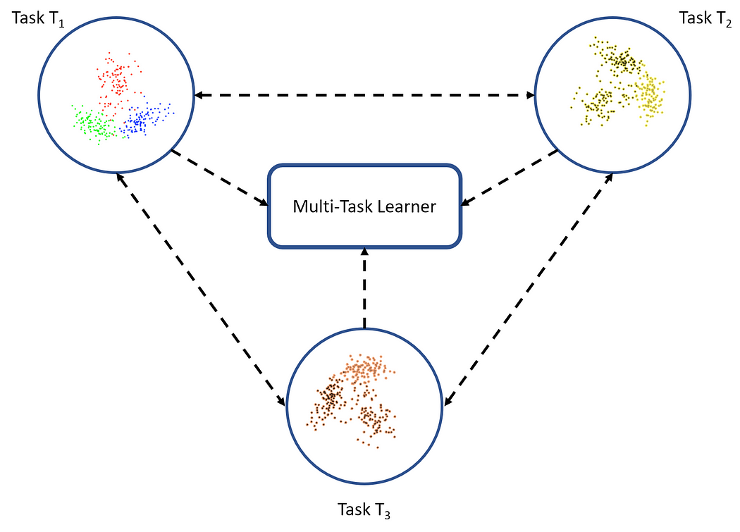
Multitask learning: Learner receives information from all tasks simultaneously
Deep learning systems are data-hungry by nature, such that they need many training examples to learn the weights. This is one of the limiting aspects of deep neural networks, though such is not the case with human learning. For instance, once a child is shown what an apple looks like, they can easily identify a different variety of apple (with one or a few training examples); this is not the case with ML and deep learning algorithms. One-shot learning is a variant of transfer learning, where we try to infer the required output based on just one or a few training examples. This is essentially helpful in real-world scenarios where it is not possible to have labeled data for every possible class (if it is a classification task), and in scenarios where new classes can be added often. This approach has since been improved upon, and applied using deep learning systems.
Zero-shot learning is another extreme variant of transfer learning, which relies on no labeled examples to learn a task. This might sound unbelievable, especially when learning using examples is what most supervised learning algorithms are about. Zero-data learning or zero-short learning methods, make clever adjustments during the training stage itself to exploit additional information to understand unseen data. In their book on Deep Learning, Goodfellow and their co-authors present zero-shot learning as a scenario where three variables are learned, such as the traditional input variable, x, the traditional output variable, y, and the additional random variable that describes the task, T. The model is thus trained to learn the conditional probability distribution of P(y | x, T). Zero-shot learning comes in handy in scenarios such as machine translation, where we may not even have labels in the target language.
Deep learning is definitely one of the specific categories of algorithms that has been utilized to reap the benefits of transfer learning very successfully. The following are a few examples:
Thus, these findings have helped in utilizing existing state-of-the-art models, such as VGG, AlexNet, and Inceptions, for target tasks, such as style transfer and face detection, that were different from what these models were trained for initially. Let’s explore some real-world case studies now and build some deep transfer learning models!
In this simple case study, will be working on an image categorization problem with the constraint of having a very small number of training samples per category. The dataset for our problem is available on Kaggle and is one of the most popular computer vision based datasets out there.
The dataset that we will be using, comes from the very popular Dogs vs. Cats Challenge, where our primary objective is to build a deep learning model that can successfully recognize and categorize images into either a cat or a dog.

To start, download the train.zip file from the dataset page and store it in your local system. Once downloaded, unzip it into a folder. This folder will contain 25,000 images of dogs and cats; that is, 12,500 images per category. While we can use all 25,000 images and build some nice models on them, if you remember, our problem objective includes the added constraint of having a small number of images per category. Let’s build our own dataset for this purpose.
import glob
import numpy as np
import os
import shutilnp.random.seed(42)
Let’s now load up all the images in our original training data folder as follows:
(12500, 12500)
We can verify with the preceding output that we have 12,500 images for each category. Let’s now build our smaller dataset, so that we have 3,000 images for training, 1,000 images for validation, and 1,000 images for our test dataset (with equal representation for the two animal categories).
Cat datasets: (1500,) (500,) (500,)
Dog datasets: (1500,) (500,) (500,)
Now that our datasets have been created, let’s write them out to our disk in separate folders, so that we can come back to them anytime in the future without worrying if they are present in our main memory.
Since this is an image categorization problem, we will be leveraging CNN models or ConvNets to try and tackle this problem. We will start by building simple CNN models from scratch, then try to improve using techniques such as regularization and image augmentation. Then, we will try and leverage pre-trained models to unleash the true power of transfer learning!
Before we jump into modeling, let’s load and prepare our datasets. To start with, we load up some basic dependencies.
import glob
import numpy as np
import matplotlib.pyplot as plt
from keras.preprocessing.image import ImageDataGenerator, load_img, img_to_array, array_to_img%matplotlib inline
Let’s now load our datasets, using the following code snippet.
Train dataset shape: (3000, 150, 150, 3)
Validation dataset shape: (1000, 150, 150, 3)
We can clearly see that we have 3000 training images and 1000 validation images. Each image is of size 150 x 150 and has three channels for red, green, and blue (RGB), hence giving each image the (150, 150, 3) dimensions. We will now scale each image with pixel values between (0, 255) to values between (0, 1) because deep learning models work really well with small input values.
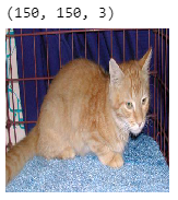
The preceding output shows one of the sample images from our training dataset. Let’s now set up some basic configuration parameters and also encode our text class labels into numeric values (otherwise, Keras will throw an error).
['cat', 'cat', 'cat', 'cat', 'cat', 'dog', 'dog', 'dog', 'dog', 'dog'] [0 0 0 0 0 1 1 1 1 1]
We can see that our encoding scheme assigns the number 0 to the cat labels and 1 to the dog labels. We are now ready to build our first CNN-based deep learning model.
We will start by building a basic CNN model with three convolutional layers, coupled with max pooling for auto-extraction of features from our images and also downsampling the output convolution feature maps.
We assume you have enough knowledge about CNNs and hence, won’t cover theoretical details. Feel free to refer to my book or any other resources on the web which explain convolutional neural networks! Let’s leverage Keras and build our CNN model architecture now.
The preceding output shows us our basic CNN model summary. Just like we mentioned before, we are using three convolutional layers for feature extraction. The flatten layer is used to flatten out 128 of the 17 x 17 feature maps that we get as output from the third convolution layer. This is fed to our dense layers to get the final prediction of whether the image should be a dog (1) or a cat (0). All of this is part of the model training process, so let’s train our model using the following snippet which leverages the fit(…) function.
The following terminology is very important with regard to training our model:
batch_size indicates the total number of images passed to the model per iteration.batch_sizeWe use a batch_size of 30 and our training data has a total of 3,000 samples, which indicates that there will be a total of 100 iterations per epoch. We train the model for a total of 30 epochs and validate it consequently on our validation set of 1,000 images.
Train on 3000 samples, validate on 1000 samples
Epoch 1/30
3000/3000 - 10s - loss: 0.7583 - acc: 0.5627 - val_loss: 0.7182 - val_acc: 0.5520
Epoch 2/30
3000/3000 - 8s - loss: 0.6343 - acc: 0.6533 - val_loss: 0.5891 - val_acc: 0.7190
...
...
Epoch 29/30
3000/3000 - 8s - loss: 0.0314 - acc: 0.9950 - val_loss: 2.7014 - val_acc: 0.7140
Epoch 30/30
3000/3000 - 8s - loss: 0.0147 - acc: 0.9967 - val_loss: 2.4963 - val_acc: 0.7220
Looks like our model is kind of overfitting, based on the training and validation accuracy values. We can plot our model accuracy and errors using the following snippet to get a better perspective.

Vanilla CNN Model Performance
You can clearly see that after 2–3 epochs the model starts overfitting on the training data. The average accuracy we get in our validation set is around 72%, which is not a bad start! Can we improve upon this model?
Let’s improve upon our base CNN model by adding in one more convolution layer, another dense hidden layer. Besides this, we will add dropout of 0.3 after each hidden dense layer to enable regularization. Basically, dropout is a powerful method of regularizing in deep neural nets. It can be applied separately to both input layers and the hidden layers. Dropout randomly masks the outputs of a fraction of units from a layer by setting their output to zero (in our case, it is 30% of the units in our dense layers).
Train on 3000 samples, validate on 1000 samples
Epoch 1/30
3000/3000 - 7s - loss: 0.6945 - acc: 0.5487 - val_loss: 0.7341 - val_acc: 0.5210
Epoch 2/30
3000/3000 - 7s - loss: 0.6601 - acc: 0.6047 - val_loss: 0.6308 - val_acc: 0.6480
...
...
Epoch 29/30
3000/3000 - 7s - loss: 0.0927 - acc: 0.9797 - val_loss: 1.1696 - val_acc: 0.7380
Epoch 30/30
3000/3000 - 7s - loss: 0.0975 - acc: 0.9803 - val_loss: 1.6790 - val_acc: 0.7840

Vanilla CNN Model with Regularization Performance
You can clearly see from the preceding outputs that we still end up overfitting the model, though it takes slightly longer and we also get a slightly better validation accuracy of around 78%, which is decent but not amazing. The reason for model overfitting is because we have much less training data and the model keeps seeing the same instances over time across each epoch. A way to combat this would be to leverage an image augmentation strategy to augment our existing training data with images that are slight variations of the existing images. We will cover this in detail in the following section. Let’s save this model for the time being so we can use it later to evaluate its performance on the test data.
model.save(‘cats_dogs_basic_cnn.h5’)
Let’s improve upon our regularized CNN model by adding in more data using a proper image augmentation strategy. Since our previous model was trained on the same small sample of data points each time, it wasn’t able to generalize well and ended up overfitting after a few epochs. The idea behind image augmentation is that we follow a set process of taking in existing images from our training dataset and applying some image transformation operations to them, such as rotation, shearing, translation, zooming, and so on, to produce new, altered versions of existing images. Due to these random transformations, we don’t get the same images each time, and we will leverage Python generators to feed in these new images to our model during training.
The Keras framework has an excellent utility called ImageDataGenerator that can help us in doing all the preceding operations. Let’s initialize two of the data generators for our training and validation datasets.
There are a lot of options available in ImageDataGenerator and we have just utilized a few of them. In our training data generator, we take in the raw images and then perform several transformations on them to generate new images. These include the following.
0.3 using the zoom_range parameter.50 degrees using the rotation_range parameter.0.2 factor of the image’s width or height using the width_shift_range and the height_shift_range parameters.shear_range parameter.horizontal_flip parameter.fill_mode parameter to fill in new pixels for images after we apply any of the preceding operations (especially rotation or translation). In this case, we just fill in the new pixels with their nearest surrounding pixel values.Let’s see how some of these generated images might look so that you can understand them better. We will take two sample images from our training dataset to illustrate the same. The first image is an image of a cat.
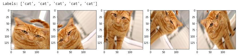
Image Augmentation on a Cat Image
You can clearly see in the previous output that we generate a new version of our training image each time (with translations, rotations, and zoom) and also we assign a label of cat to it so that the model can extract relevant features from these images and also remember that these are cats. Let’s look at how image augmentation works on a sample dog image now.

Image Augmentation on a Dog Image
This shows us how image augmentation helps in creating new images, and how training a model on them should help in combating overfitting. Remember for our validation generator, we just need to send the validation images (original ones) to the model for evaluation; hence, we just scale the image pixels (between 0–1) and do not apply any transformations. We just apply image augmentation transformations only on our training images. Let’s now train a CNN model with regularization using the image augmentation data generators we created. We will use the same model architecture from before.
We reduce the default learning rate by a factor of 10 here for our optimizer to prevent the model from getting stuck in a local minima or overfit, as we will be sending a lot of images with random transformations. To train the model, we need to slightly modify our approach now, since we are using data generators. We will leverage the fit_generator(…) function from Keras to train this model. The train_generator generates 30 images each time, so we will use the steps_per_epoch parameter and set it to 100 to train the model on 3,000 randomly generated images from the training data for each epoch. Our val_generator generates 20 images each time so we will set the validation_steps parameter to 50 to validate our model accuracy on all the 1,000 validation images (remember we are not augmenting our validation dataset).
Epoch 1/100
100/100 - 12s - loss: 0.6924 - acc: 0.5113 - val_loss: 0.6943 - val_acc: 0.5000
Epoch 2/100
100/100 - 11s - loss: 0.6855 - acc: 0.5490 - val_loss: 0.6711 - val_acc: 0.5780
Epoch 3/100
100/100 - 11s - loss: 0.6691 - acc: 0.5920 - val_loss: 0.6642 - val_acc: 0.5950
...
...
Epoch 99/100
100/100 - 11s - loss: 0.3735 - acc: 0.8367 - val_loss: 0.4425 - val_acc: 0.8340
Epoch 100/100
100/100 - 11s - loss: 0.3733 - acc: 0.8257 - val_loss: 0.4046 - val_acc: 0.8200
We get a validation accuracy jump to around 82%, which is almost 4–5% better than our previous model. Also, our training accuracy is very similar to our validation accuracy, indicating our model isn’t overfitting anymore. The following depict the model accuracy and loss per epoch.
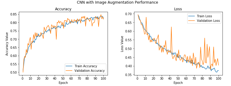
Vanilla CNN Model with Image Augmentation Performance
While there are some spikes in the validation accuracy and loss, overall, we see that it is much closer to the training accuracy, with the loss indicating that we obtained a model that generalizes much better as compared to our previous models. Let’s save this model now so we can evaluate it later on our test dataset.
model.save(‘cats_dogs_cnn_img_aug.h5’)
We will now try and leverage the power of transfer learning to see if we can build a better model!
Pre-trained models are used in the following two popular ways when building new models or reusing them:
A pre-trained model like the VGG-16 is an already pre-trained model on a huge dataset (ImageNet) with a lot of diverse image categories. Considering this fact, the model should have learned a robust hierarchy of features, which are spatial, rotation, and translation invariant with regard to features learned by CNN models. Hence, the model, having learned a good representation of features for over a million images belonging to 1,000 different categories, can act as a good feature extractor for new images suitable for computer vision problems. These new images might never exist in the ImageNet dataset or might be of totally different categories, but the model should still be able to extract relevant features from these images.
This gives us an advantage of using pre-trained models as effective feature extractors for new images, to solve diverse and complex computer vision tasks, such as solving our cat versus dog classifier with fewer images, or even building a dog breed classifier, a facial expression classifier, and much more! Let’s briefly discuss the VGG-16 model architecture before unleashing the power of transfer learning on our problem.
The VGG-16 model is a 16-layer (convolution and fully connected) network built on the ImageNet database, which is built for the purpose of image recognition and classification. This model was built by Karen Simonyan and Andrew Zisserman.
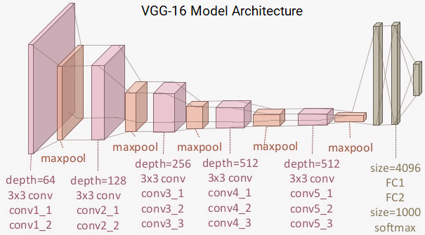
VGG-16 Model Architecture
You can clearly see that we have a total of 13 convolution layers using 3 x 3 convolution filters along with max pooling layers for downsampling and a total of two fully connected hidden layers of 4096 units in each layer followed by a dense layer of 1000 units, where each unit represents one of the image categories in the ImageNet database. We do not need the last three layers since we will be using our own fully connected dense layers to predict whether images will be a dog or a cat. We are more concerned with the first five blocks, so that we can leverage the VGG model as an effective feature extractor.
For one of the models, we will use it as a simple feature extractor by freezing all the five convolution blocks to make sure their weights don’t get updated after each epoch. For the last model, we will apply fine-tuning to the VGG model, where we will unfreeze the last two blocks (Block 4 and Block 5) so that their weights get updated in each epoch (per batch of data) as we train our own model. We represent the preceding architecture, along with the two variants (basic feature extractor and fine-tuning) that we will be using, in the following block diagram, so you can get a better visual perspective.

Block Diagram showing Transfer Learning Strategies on the VGG-16 Model
Thus, we are mostly concerned with leveraging the convolution blocks of the VGG-16 model and then flattening the final output (from the feature maps) so that we can feed it into our own dense layers for our classifier.
Let’s leverage Keras, load up the VGG-16 model, and freeze the convolution blocks so that we can use it as just an image feature extractor.
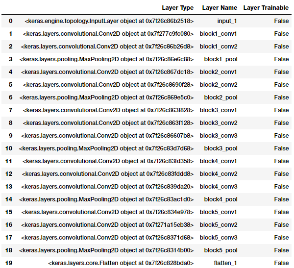
It is quite clear from the preceding output that all the layers of the VGG-16 model are frozen, which is good, because we don’t want their weights to change during model training. The last activation feature map in the VGG-16 model (output from block5_pool) gives us the bottleneck features, which can then be flattened and fed to a fully connected deep neural network classifier. The following snippet shows what the bottleneck features look like for a sample image from our training data.
bottleneck_feature_example = vgg.predict(train_imgs_scaled[0:1])
print(bottleneck_feature_example.shape)
plt.imshow(bottleneck_feature_example[0][:,:,0])
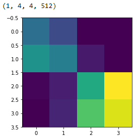
Sample Bottleneck Features
We flatten the bottleneck features in the vgg_model object to make them ready to be fed to our fully connected classifier. A way to save time in model training is to use this model and extract out all the features from our training and validation datasets and then feed them as inputs to our classifier. Let’s extract out the bottleneck features from our training and validation sets now.
Train Bottleneck Features: (3000, 8192)
Validation Bottleneck Features: (1000, 8192)
The preceding output tells us that we have successfully extracted the flattened bottleneck features of dimension 1 x 8192 for our 3,000 training images and our 1,000 validation images. Let’s build the architecture of our deep neural network classifier now, which will take these features as input.
Just like we mentioned previously, bottleneck feature vectors of size 8192 serve as input to our classification model. We use the same architecture as our previous models here with regard to the dense layers. Let’s train this model now.
Train on 3000 samples, validate on 1000 samples
Epoch 1/30
3000/3000 - 1s 373us/step - loss: 0.4325 - acc: 0.7897 - val_loss: 0.2958 - val_acc: 0.8730
Epoch 2/30
3000/3000 - 1s 286us/step - loss: 0.2857 - acc: 0.8783 - val_loss: 0.3294 - val_acc: 0.8530
Epoch 3/30
3000/3000 - 1s 289us/step - loss: 0.2353 - acc: 0.9043 - val_loss: 0.2708 - val_acc: 0.8700
...
...
Epoch 29/30
3000/3000 - 1s 287us/step - loss: 0.0121 - acc: 0.9943 - val_loss: 0.7760 - val_acc: 0.8930
Epoch 30/30
3000/3000 - 1s 287us/step - loss: 0.0102 - acc: 0.9987 - val_loss: 0.8344 - val_acc: 0.8720

Pre-trained CNN (feature extractor) Performance
We get a model with a validation accuracy of close to 88%, almost a 5–6% improvement from our basic CNN model with image augmentation, which is excellent. The model does seem to be overfitting though. There is a decent gap between the model train and validation accuracy after the fifth epoch, which kind of makes it clear that the model is overfitting on the training data after that. But overall, this seems to be the best model so far. Let’s try using our image augmentation strategy on this model. Before that, we save this model to disk using the following code.
model.save('cats_dogs_tlearn_basic_cnn.h5')
We will leverage the same data generators for our train and validation datasets that we used before. The code for building them is depicted as follows for ease of understanding.
Let’s now build our deep learning model and train it. We won’t extract the bottleneck features like last time since we will be training on data generators; hence, we will be passing the vgg_model object as an input to our own model. We bring the learning rate slightly down since we will be training for 100 epochs and don’t want to make any sudden abrupt weight adjustments to our model layers. Do remember that the VGG-16 model’s layers are still frozen here, and we are still using it as a basic feature extractor only.
Epoch 1/100
100/100 - 45s 449ms/step - loss: 0.6511 - acc: 0.6153 - val_loss: 0.5147 - val_acc: 0.7840
Epoch 2/100
100/100 - 41s 414ms/step - loss: 0.5651 - acc: 0.7110 - val_loss: 0.4249 - val_acc: 0.8180
Epoch 3/100
100/100 - 41s 415ms/step - loss: 0.5069 - acc: 0.7527 - val_loss: 0.3790 - val_acc: 0.8260
...
...
Epoch 99/100
100/100 - 42s 417ms/step - loss: 0.2656 - acc: 0.8907 - val_loss: 0.2757 - val_acc: 0.9050
Epoch 100/100
100/100 - 42s 418ms/step - loss: 0.2876 - acc: 0.8833 - val_loss: 0.2665 - val_acc: 0.9000

Pre-trained CNN (feature extractor) with Image Augmentation Performance
We can see that our model has an overall validation accuracy of 90%, which is a slight improvement from our previous model, and also the train and validation accuracy are quite close to each other, indicating that the model is not overfitting. Let’s save this model on the disk now for future evaluation on the test data.
model.save(‘cats_dogs_tlearn_img_aug_cnn.h5’)
We will now fine-tune the VGG-16 model to build our last classifier, where we will unfreeze blocks 4 and 5, as we depicted in our block diagram earlier.
We will now leverage our VGG-16 model object stored in the vgg_model variable and unfreeze convolution blocks 4 and 5 while keeping the first three blocks frozen. The following code helps us achieve this.
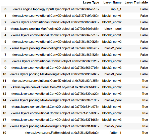
You can clearly see from the preceding output that the convolution and pooling layers pertaining to blocks 4 and 5 are now trainable. This means the weights for these layers will also get updated with backpropagation in each epoch as we pass each batch of data. We will use the same data generators and model architecture as our previous model and train our model. We reduce the learning rate slightly, since we don’t want to get stuck at any local minimal, and we also do not want to suddenly update the weights of the trainable VGG-16 model layers by a big factor that might adversely affect the model.
Epoch 1/100
100/100 - 64s 642ms/step - loss: 0.6070 - acc: 0.6547 - val_loss: 0.4029 - val_acc: 0.8250
Epoch 2/100
100/100 - 63s 630ms/step - loss: 0.3976 - acc: 0.8103 - val_loss: 0.2273 - val_acc: 0.9030
Epoch 3/100
100/100 - 63s 631ms/step - loss: 0.3440 - acc: 0.8530 - val_loss: 0.2221 - val_acc: 0.9150
...
...
Epoch 99/100
100/100 - 63s 629ms/step - loss: 0.0243 - acc: 0.9913 - val_loss: 0.2861 - val_acc: 0.9620
Epoch 100/100
100/100 - 63s 629ms/step - loss: 0.0226 - acc: 0.9930 - val_loss: 0.3002 - val_acc: 0.9610
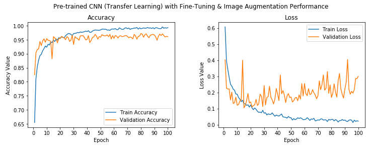
Pre-trained CNN (fine-tuning) with Image Augmentation Performance
We can see from the preceding output that our model has obtained a validation accuracy of around 96%, which is a 6% improvement from our previous model. Overall, this model has gained a 24% improvement in validation a


 Comment


Vibhuti kumar 22 Sep, 2022
What if i want to classify a larger input image,what should i do after changed the input shape from fixed 224x224 to sth like 896x896,add some new layer to reduce final output feature maps?Thank you,anyway,your post is of great help to understand transfer learning!
Swati 22 Sep, 2022
For the case study 1 about the dog/cat classification, did you try to fit a model similar to the model 5 ( i.e. Pre-trained CNN with Fine-tuning and Image Augmentation Performance) but with a random initialization of weights of the vgg part, and with setting every layers of the vgg part as trainable, in order to evaluate the impact of transfer learning on a specific model ?